This article is the second part of a complete installment on the in-depth analysis of capacitor losses. It focus on the role of Equivalent Series Resistance (ESR), Dissipation Factor (DF or tanδ), and Quality Factor (Q). It explores how losses shift between series and parallel circuit models depending on frequency, with ESR dominating at high frequencies and parallel resistance (Rp) taking precedence at low frequencies. The discussion includes the transition of impedance behavior across frequencies, the significance of Q values in high-frequency applications, and an analysis of dielectric losses, electrode contributions, and equivalent circuit models to provide a comprehensive understanding of capacitor performance.
The complete analysis is divided in 4 stages:
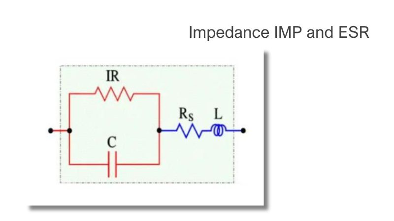
- Impedance IMP and ESR
- Dissipation Factor (DF) / Tanδ and Q Value
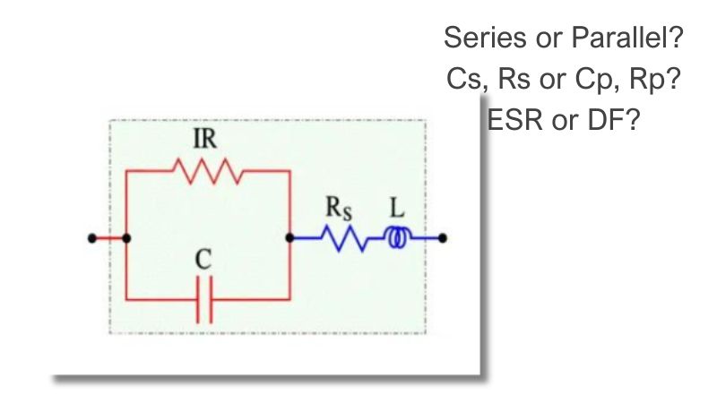
- Series or Parallel? Cs, Rs or Cp, Rp? ESR or DF?
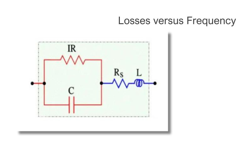
- Losses versus Frequency
Dissipation Factor (DF) / Tanδ and Q Value
The losses in Figure 6. are concentrated in the ESR, which becomes significant when we leave the low-frequency range. For HF chips and high-loss components for example, electrolytes often the ESR is stated in the data sheets. If the ESR information is missing, you always find, for all component types, a specified dissipation factor (DF), the tanδ (Figure 6).
Hence, at higher frequencies, the series circuit, according to Figure 3, applies. There is

……………….. [4]
Tanδ usually is expressed in %.
If the frequency declines to zero, the circuit becomes resistive, without any capacitance, and the losses are limited to the IR. Also, at very low frequencies, the IR is predominant, but here it should be completed with dawning AC-dependent losses to an equivalent loss resistance Rp. The diagram in Figure 2. can now be simplified to a parallel circuit with the capacitance Cp (Figure 7.).

Figure 6. Definition of Tanδ in a series circuit

Figure 7. The equivalent parallel circuit of a capacitor. Applies at low frequencies
If we describe the impedance in a parallel circuit according to Figure 7. it’s easy to show that its dissipation factor – which applies at low frequencies – can be written as

……………………………[5]
The difference between Cs and Cp usually is negligible depending on the impedance value – see note below. We shall return to the connections in some formulas. If we equate the formula [2] with [3], we obtain


……………………[6]
Let us terminate the discussion about the capacitor losses by distinguishing the different types of losses as in the following Figure 8.
Q value Dielectric Quality Factor
Sometimes we encounter the Q or Q value, especially in high-frequency applications. Instead of describing the capacitor losses as DF (Tanδ) we rather specify its freedom from losses, its figure of merit, the Q value. It is defined as

……………………………[7]
Typical Q values for ceramic Class 1 dielectric range from 200 to 2000 at 100 MHz and will vary strongly with frequency.
We shall use the Q value to describe the connection between the quantities in the series and parallel circuits in Figures C1-18 and -20. By depicting the expressions for the impedance and Q values of these circuits and equating the real and imaginary parts of the impedance, we can show that

………………………………[8]

………………………………[9]

………………………………[10]

………………………………[11]

Figure 8. Equivalent diagram with dielectric losses particularly marked
- Rd = dielectric losses
- Rs = losses in leading-in wires, joints and electrode metallizations
- ESR = Rs + Rd
- C = C1 + C2.
Related Articles
Impedance IMP and ESR
Series or Parallel? Cs, Rs or Cp, Rp? ESR or DF?